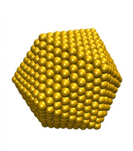
This example will walk you through how to build an icosahedral gold nanoparticle and equilibrate the system to 250K.
Here we will be building an icosahedra with 8 shells (layers of gold atoms). Icosahedra are experimentally interesting due to the 20 exposed (111) facets, which have a lower surface energy than exhibited by the spherical particles.
- To start the process, a metal file (gold.omd) is needed to describe the material composition of the particle. We will take the same file from Building and equilibrating a gold nanoparticle in OpenMD
molecule{
name = "Au";
atom[0]{
type = "Au";
position(0.0, 0.0, 0.0);
}
}
component{
type = "Au";
nMol = 1;
}
forceField = "SC";
forceFieldFileName = "SuttonChen.QSC.frc"; - To create the particle coordinates, use the command:
icosahedralBuilder -o file.omd --shell=8 --latticeConstant=4.08 --ico gold.omd
where file.omd is the name of your icosahedra, 8 is the number of shells (in this example), 4.08 is the lattice constant in Angstroms for the metal (4.08 is the correct value for gold), and the skeletal OpenMD file above is called gold.omd
- To make sure this icosahedra is the right size for your purposes; use Dump2XYZ to create an xyz file:
Dump2XYZ -i file.omd
and view the file in VMD or Jmol (where you might want to measure the diameter of the particle).
- To run the icosahedra in a Langevin Hull and heat the system, we’ll start by inserting the following excerpt after the forceFieldFileName in file.omd.
ensemble = "LHull";
targetTemp = 5;
targetPressure = 1;
viscosity = 0.1;
dt = 4.0;
runTime = 2E5;
sampleTime = 2000.0;
statusTime = 4;
seed = 985456376;
usePeriodicBoundaryConditions = "false";
tauThermostat = 1E3;
tauBarostat = 5E3; - Before we can equilibrate the system, the atoms need initial velocities, which we can set using the thermalizer command.
thermalizer -t 5 -o file-5K.omd file.omd
where -t is followed by the desired temperature in Kelvin, and -o is followed by the output file name.
- To relax the particle at 5K, we’ll run the simulation described in file-5K.omd using the openmd command:
openmd file-5K.omd
- To ensure that the temperature of the system has reached 5K, we can use xmgrace to view the stat file:
xmgrace -nxy file-5K.stat
In a typical stat file, set 3 (the fourth column) contains the information about the temperature of the system. You can view only the temperature for the trajectory by double clicking any line and bringing up the Set Appearance box. All the sets are initially displayed; turn off the sets you don’t want to see by highlighting and right clicking the set to click the Hide option.
- The “end of run” file that has been relaxed can then be copied to a new simulation that will be heated to 100K.
cp file-5K.eor file-100K.omd
Then change the targetTemp from 5 to 100.
- We’ll continue the procedure of copying the .eor file to a new .omd file and increasing the temperature until we’ve reached 250K. Temperature increases of 50 – 100K and simulation times of 100 – 200 ps are reasonable. Heating the system in intervals is relatively effective in keeping the geometry of the particle stable.
#1 by kedar on June 30, 2017 - 10:06 am
Warning: Undefined variable $my_comment_count in /Users/Gezelter/openmd/wordpress/wp-content/themes/arclite/functions.php on line 714
Quote
how can i convert file.xyz to file.pdb?
#2 by Dan Gezelter on July 4, 2017 - 11:57 am
Warning: Undefined variable $my_comment_count in /Users/Gezelter/openmd/wordpress/wp-content/themes/arclite/functions.php on line 714
Quote
You can use openbabel to convert between chemical file types.
#3 by Hirak on March 10, 2018 - 9:37 am
Warning: Undefined variable $my_comment_count in /Users/Gezelter/openmd/wordpress/wp-content/themes/arclite/functions.php on line 714
Quote
Is it possible to convert .xyz file to .omd file?
#4 by Marianna Kotzabasaki on May 21, 2019 - 8:59 am
Warning: Undefined variable $my_comment_count in /Users/Gezelter/openmd/wordpress/wp-content/themes/arclite/functions.php on line 714
Quote
How can i convert .xyz file to .omd file?
#5 by Dan Gezelter on May 21, 2019 - 9:43 am
Warning: Undefined variable $my_comment_count in /Users/Gezelter/openmd/wordpress/wp-content/themes/arclite/functions.php on line 714
Quote
Marianna,
If OpenMD was built with the openbabel library support, there should be a program called “atom2omd” in the installation. You can use it as follows:
Note that most of the converted files will need significant editing before they can be used by OpenMD. You’ll have to set a force field, and edit the atom types at a minimum, but the coordinates should get converted into the correct format.
#6 by sokeym on May 31, 2019 - 11:29 am
Warning: Undefined variable $my_comment_count in /Users/Gezelter/openmd/wordpress/wp-content/themes/arclite/functions.php on line 714
Quote
Hello how can a build a 60nm gold nanoparticle modified with ligands
#7 by Dan Gezelter on May 31, 2019 - 8:23 pm
Warning: Undefined variable $my_comment_count in /Users/Gezelter/openmd/wordpress/wp-content/themes/arclite/functions.php on line 714
Quote
I answered this partially on another post, but that’s a very large particle (roughly 52 million atoms). Are you sure you want to do this?
#8 by Kwasi Kantanka Safo on August 23, 2023 - 6:05 am
Warning: Undefined variable $my_comment_count in /Users/Gezelter/openmd/wordpress/wp-content/themes/arclite/functions.php on line 714
Quote
Sir, please can you help me design a silver nanoparticle… I have no knowledge in using python… But I’d like to perform in silico test on how to detect several drugs using silver nanomaterial
#9 by Dan Gezelter on August 23, 2023 - 10:12 am
Warning: Undefined variable $my_comment_count in /Users/Gezelter/openmd/wordpress/wp-content/themes/arclite/functions.php on line 714
Quote
Silver and Gold have very similar lattice constants, so you can use the same procedure as above with “Ag” replacing “Au” to create a silver nanoparticle. If you want to use OpenMD, then you’ll want to narrowly define what you mean by ‘detecting drugs’ into something that can be answered via a molecular dynamics simulation.